Orbital classify

Orbit classification based on the resonance angle behaviour.

import numpy as np
import matplotlib.pyplot as plt

import galport

Load coordinates, velocities and actions for the set of orbits

xv_act = np.load('data/xv_act_0.npy')

t = np.arange(0, 600.125, 0.125)
xv = xv_act[:,:,0:6]
act = xv_act[:,:,6:9]

theta_p = np.load('data/phi_p.npy')
Omega_p = np.load('data/omega_p.npy')

Find actions, angles and frequencies of the every orbit and Orbit classification at time \(t=400\)

%%time

OT = galport.OrbitTools(t=t, xv=xv, act=act)
data = OT.calculate_actions(secular=True, parallel=True)

CPU times: user 228 ms, sys: 129 ms, total: 357 ms
Wall time: 650 ms

%%time

otype_ILR = OT.classify_orbits(t_out=400, family='ILR', theta_p=theta_p)
otype_vILR = OT.classify_orbits(t_out=400, family='vILR', theta_p=theta_p)
otype_uha = OT.classify_orbits(t_out=400, family='uha', theta_p=theta_p)

CPU times: user 42.3 ms, sys: 8.11 ms, total: 50.4 ms
Wall time: 49.5 ms

Equivalent code for classification (calling the OrbitClassifier module directly)

ang = OT.angles
# or
ang = data[:, :, 3:6] # if dJdt=False
# ang = OT.data[:, :, 6:9] # if dJdt=True

OC = galport.OrbitClassifier(t, angles=ang, theta_p=theta_p, time_resolution=5.)
# Not all angles are used in the classification; they are taken with a time step of `time_resolution`
result = OC(t_out=400, family='ILR', time_around_res=False, amplitude_res=False)
# or, you can also set the resonant angle yourself
OC = galport.OrbitClassifier(t, angles=2*(ang[:,:,2] - theta_p) - ang[:,:,0], time_resolution=5.)
result = OC(t_out=400, time_around_res=True, amplitude_res=False)

List of types

0: Not classify

1: Increasing angle

2: Decreasing angle

3: Resonance around \(0\)

4: Resonance around \(\pi\)

5: Passage through \(0\) from \(\Omega_{res} > 0\) to \(\Omega_{res} < 0\)

6: Passage through \(\pi\) from \(\Omega_{res} > 0\) to \(\Omega_{res} < 0\)

7: Passage through \(0\) from \(\Omega_{res} < 0\) to \(\Omega_{res} > 0\)

8: Passage through \(\pi\) from \(\Omega_{res} < 0\) to \(\Omega_{res} > 0\)

Additional variables

time_around_res: returns the resonance entry and exit times for resonant orbits

amplitude_res: returns the maximum libration amplitude of the resonant angle

Secular actions and frequencies

t0 = 400
n_t = int(t0)*8

JR_sec = data[:,n_t,9]
Jz_sec = data[:,n_t,10]
Lz_sec = data[:,n_t,11]

kappa_sec = data[:,n_t,12]
omegaz_sec = data[:,n_t,13]
Omega_sec = data[:,n_t,14] - Omega_p[n_t]

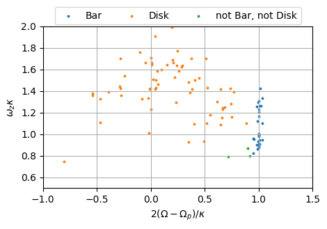
Plot different orbital types on the plane \(2(\Omega - \Omega_p)/\kappa\) vs \(\omega_z\kappa\)

fig, ax = plt.subplots(figsize=(5,5))
ax.set_aspect('equal')

ax.grid(zorder=-1)

test_bar = (otype_ILR > 2)
test_notbarnotdisk = (otype_ILR <= 2) & (otype_uha == 1) & (otype_vILR == 2)
test_disk = ~test_bar & ~test_notbarnotdisk


ax.scatter(
    2*Omega_sec[test_bar]/kappa_sec[test_bar],
    omegaz_sec[test_bar]/kappa_sec[test_bar],
    s=3, label='Bar'
)

ax.scatter(
    2*Omega_sec[test_disk]/kappa_sec[test_disk],
    omegaz_sec[test_disk]/kappa_sec[test_disk],
    s=3, label='Disk'
)

ax.scatter(
    2*Omega_sec[test_notbarnotdisk]/kappa_sec[test_notbarnotdisk],
    omegaz_sec[test_notbarnotdisk]/kappa_sec[test_notbarnotdisk],
    s=3, label='not Bar, not Disk'
)


ax.set_xlabel('$2(\\Omega - \\Omega_p)/\\kappa$')
ax.set_ylabel('$\\omega_z\\kappa$')
ax.legend(
    loc='upper center',
    bbox_to_anchor=(0.5, 1.15),
    ncols=3
)

ax.set_xlim(-1.0,1.5)
ax.set_ylim(0.5, 2)

plt.show()

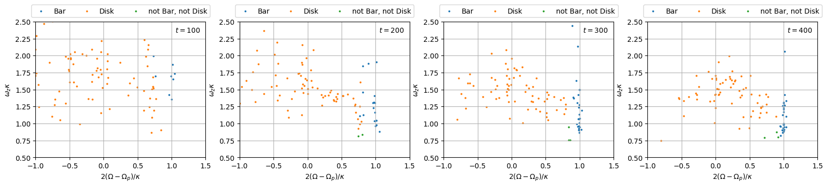
Orbits can be classified at different points in time. Classification for each point in time is parallelised.

%%time
t_out = np.arange(100, 505, 5)
otypes_ILR = OT.classify_orbits(t_out=t_out, family='ILR', theta_p=theta_p, parallel=True, n_jobs=4)
otypes_vILR = OT.classify_orbits(t_out=t_out, family='vILR', theta_p=theta_p, parallel=True, n_jobs=4)
otypes_uha = OT.classify_orbits(t_out=t_out, family='uha', theta_p=theta_p, parallel=True, n_jobs=4)

CPU times: user 57.1 ms, sys: 166 ms, total: 223 ms
Wall time: 692 ms

%%time
t_out = np.arange(100, 505, 5)
otypes_ILR = OT.classify_orbits(t_out=t_out, family='ILR', theta_p=theta_p, parallel=False)
otypes_vILR = OT.classify_orbits(t_out=t_out, family='vILR', theta_p=theta_p, parallel=False)
otypes_uha = OT.classify_orbits(t_out=t_out, family='uha', theta_p=theta_p, parallel=False)

CPU times: user 1.45 s, sys: 4.6 ms, total: 1.46 s
Wall time: 1.46 s

fig, axes = plt.subplots(1, 4, figsize=(20,5))

i_plot = [0, 20, 40, 60]
t_plot = t_out[i_plot]
for j, (i, t) in enumerate(zip(i_plot, t_plot)):
    ax = axes[j]
    otype_ILR = otypes_ILR[i]
    otype_uha = otypes_uha[i]
    otype_vILR = otypes_vILR[i]

    n_t = int(t)*8
    JR_sec = data[:,n_t,9]
    Jz_sec = data[:,n_t,10]
    Lz_sec = data[:,n_t,11]

    kappa_sec = data[:,n_t,12]
    omegaz_sec = data[:,n_t,13]
    Omega_sec = data[:,n_t,14] - Omega_p[n_t]

    ax.set_aspect('equal')

    ax.grid(zorder=-1)

    test_bar = (otype_ILR > 2)
    test_notbarnotdisk = (otype_ILR <= 2) & (otype_uha == 1) & (otype_vILR == 2)
    test_disk = ~test_bar & ~test_notbarnotdisk


    ax.scatter(
        2*Omega_sec[test_bar]/kappa_sec[test_bar],
        omegaz_sec[test_bar]/kappa_sec[test_bar],
        s=3, label='Bar'
    )

    ax.scatter(
        2*Omega_sec[test_disk]/kappa_sec[test_disk],
        omegaz_sec[test_disk]/kappa_sec[test_disk],
        s=3, label='Disk'
    )

    ax.scatter(
        2*Omega_sec[test_notbarnotdisk]/kappa_sec[test_notbarnotdisk],
        omegaz_sec[test_notbarnotdisk]/kappa_sec[test_notbarnotdisk],
        s=3, label='not Bar, not Disk'
    )


    ax.set_xlabel('$2(\\Omega - \\Omega_p)/\\kappa$')
    ax.set_ylabel('$\\omega_z\\kappa$')
    ax.legend(
        loc='upper center',
        bbox_to_anchor=(0.5, 1.15),
        ncols=3
    )

    ax.text(
        0.82, 0.92, f"$t={t}$",
        transform=ax.transAxes
    )


    ax.set_xlim(-1.0,1.5)
    ax.set_ylim(0.5, 2.5)

plt.show()