Orbital tools
The galport.OrbitTools module is designed for analysing orbital datasets in the action-angle space. The orbits are derived either from high-resolution N-body simulations or from specific initial conditions integrated within a potential. Also, the module allows calculating frequencies using naif package and is connected with the module galport.OrbitClassifier classifies the orbits’ set.
[1]:
import numpy as np
import matplotlib.pyplot as plt

import galport
import agama
Load coordinates, velocities and actions for the set of orbits
[2]:
xv_act = np.load('data/xv_act_0.npy')

t = np.arange(0, 600.125, 0.125)
xv = xv_act[:,:,0:6]
act = xv_act[:,:,6:9]
Find actions, angles and frequencies of the set of orbits if their coordinates are known.
[3]:
%%time

# 100 orbits
OT = galport.OrbitTools(t=t, xv=xv, act=act)
data = OT.calculate_actions(secular=True, secular_extrema=True, secular_act_freq=True, parallel=False)
CPU times: user 3.1 s, sys: 40 ms, total: 3.14 s
Wall time: 3.14 s
[4]:
%%time
# Example of parallel calculations
# 100 orbits
OT = galport.OrbitTools(t=t, xv=xv, act=act)
data = OT.calculate_actions(secular=True, parallel=True, n_jobs=8)
CPU times: user 113 ms, sys: 122 ms, total: 235 ms
Wall time: 761 ms
[5]:
t0 = 400
n_t = int(t0)*8

JR = data[:,n_t,0]
Jz = data[:,n_t,1]
Lz = data[:,n_t,2]

JR_sec = data[:,n_t,9]
Jz_sec = data[:,n_t,10]
Lz_sec = data[:,n_t,11]

kappa = data[:,n_t,6]
omegaz = data[:,n_t,7]
Omega = data[:,n_t,8]

kappa_sec = data[:,n_t,12]
omegaz_sec = data[:,n_t,13]
Omega_sec = data[:,n_t,14]
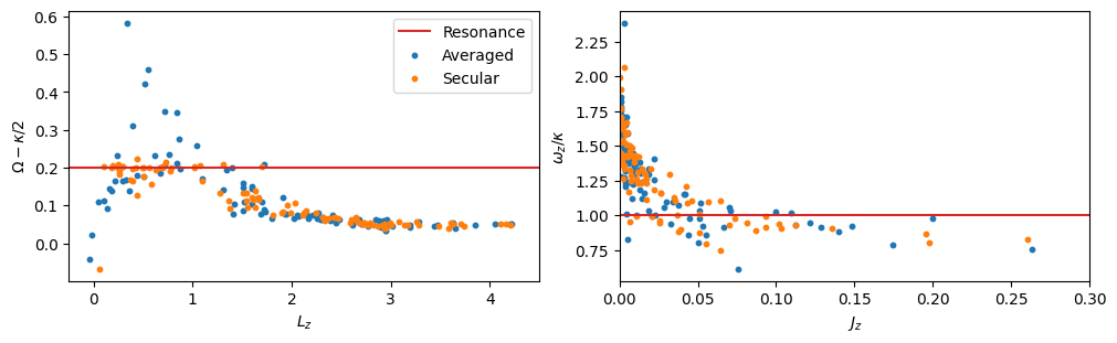
[6]:
fig, axes = plt.subplots(1, 2, figsize=(10,3), constrained_layout=True)

axes[0].plot([-0.25, 4.5], [0.2,0.2], color='C3', label='Resonance')
axes[0].scatter(Lz, Omega - kappa/2, s=10, label='Averaged')
axes[0].scatter(Lz_sec, Omega_sec - kappa_sec/2, s=10, label='Secular')
axes[0].set_xlabel('$L_z$')
axes[0].set_ylabel('$\\Omega - \\kappa/2$')
axes[0].set_xlim(-0.25, 4.5)
axes[0].legend()

axes[1].plot([0., 0.3], [1,1], color='C3')
axes[1].scatter(Jz, omegaz/kappa, s=10)
axes[1].scatter(Jz_sec, omegaz_sec/kappa_sec, s=10)
axes[1].set_xlabel('$J_z$')
axes[1].set_ylabel('$\\omega_z/\\kappa$')
axes[1].set_xlim(0, 0.3)

plt.show()
Find actions, angles and frequencies of the set of orbits. In this case, the potential, the pattern speed and initial conditions ar known. Orbits are integrated forward and backward in time if reverse=True.
[7]:
%%time

pot_gal = agama.Potential(file='data/Pot_non_CylSpline_t400.ini')
pot_gal_sym = agama.Potential(file='data/Pot_axi_CylSpline_t400.ini')

Omega = np.load('data/omega_p.npy')[400*8]
phi = -np.load('data/phi_p.npy')[400*8]

# Rotate coordinates and velocities
xv0 = xv[:,400*8].copy()
x0 = xv0[:, 0].copy()
y0 = xv0[:, 1].copy()
vx0 = xv0[:, 3].copy()
vy0 = xv0[:, 4].copy()

xv0[:, 0] = x0*np.cos(phi) - y0*np.sin(phi)
xv0[:, 1] = x0*np.sin(phi) + y0*np.cos(phi)
xv0[:, 3] = vx0*np.cos(phi) - vy0*np.sin(phi)
xv0[:, 4] = vx0*np.sin(phi) + vy0*np.cos(phi)

OT_int = galport.OrbitTools(
    xv0=xv0,
    Tint=100,
    Nint=1000,
    potential=pot_gal,
    axisym_potential=pot_gal_sym,
    reverse=True,
    Omega=Omega
)
100 orbits complete (71.68 orbits/s)
100 orbits complete (68.73 orbits/s)
CPU times: user 48.4 s, sys: 46.1 ms, total: 48.5 s
Wall time: 3.45 s
[8]:
%%time
data_int = OT_int.calculate_actions(secular=True, sidereal=True, parallel=True)
CPU times: user 126 ms, sys: 92.7 ms, total: 219 ms
Wall time: 323 ms
Comparison of actions for individual orbits obtained from N-body simulations and integration in a fixed potential.
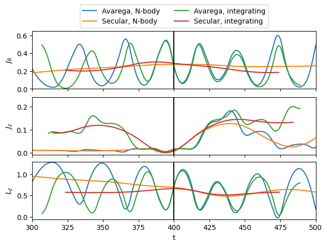
Comparison of the individual orbits
Actions for individual orbits obtained from N-body simulations and integration in a fixed potential.
[9]:
num = 7

# Actions

fig, axes = plt.subplots(3, constrained_layout=True, sharex=True)

# JR
JR = data[num,:,0]
JR_sec = data[num,:,9]
axes[0].plot(t, JR, label='Avarega, N-body')
axes[0].plot(t, JR_sec, label='Secular, N-body')
JR_int = data_int[num,:,0]
JR_sec_int = data_int[num,:,9]
axes[0].plot(OT_int.t + 400, JR_int, label='Avarega, integrating')
axes[0].plot(OT_int.t + 400, JR_sec_int, label='Secular, integrating')
axes[0].set_ylabel('$J_R$')
axes[0].set_xlim(300,500)
axes[0].plot([400,400], [-1,2], color='black')
axes[0].set_ylim(0, 1.2*np.nanmax(JR_int))
axes[0].legend(loc='lower center', bbox_to_anchor=(0.5, 1.0), ncol=2)

# Jz
Jz = data[num,:,1]
Jz_sec = data[num,:,10]
axes[1].plot(t, Jz)
axes[1].plot(t, Jz_sec)
Jz_int = data_int[num,:,1]
Jz_sec_int = data_int[num,:,10]
axes[1].plot(OT_int.t + 400, Jz_int)
axes[1].plot(OT_int.t + 400, Jz_sec_int)

axes[1].set_ylabel('$J_z$')
axes[1].set_xlim(300,500)
axes[1].plot([400,400], [-1,2], color='black')
axes[1].set_ylim(-0.01, 1.2*np.nanmax(Jz_int))

# Lz
Lz = data[num,:,2]
Lz_sec = data[num,:,11]
axes[2].plot(t, Lz)
axes[2].plot(t, Lz_sec)
Lz_int = data_int[7,:,2]
Lz_sec_int = data_int[7,:,11]
axes[2].plot(OT_int.t + 400, Lz_int)
axes[2].plot(OT_int.t + 400, Lz_sec_int)

axes[2].set_ylabel('$L_z$')
axes[2].set_xlabel('t')
axes[2].set_xlim(300,500)
axes[2].plot([400,400], [-1,2], color='black')
axes[2].set_ylim(np.nanmin(Lz_int)-0.1, 1.2*np.nanmax(Lz_int))

plt.show()
Comparison of the set of orbits
Actions and frequencies at the middle of integretion time
[10]:
n_t = (len(OT_int.t) // 2)

JR_int = data_int[:,n_t,0]
Jz_int = data_int[:,n_t,1]
Lz_int = data_int[:,n_t,2]

JR_sec_int = data_int[:,n_t,9]
Jz_sec_int = data_int[:,n_t,10]
Lz_sec_int = data_int[:,n_t,11]

kappa_int = data_int[:,n_t,6]
omegaz_int = data_int[:,n_t,7]
Omega_int = data_int[:,n_t,8]

kappa_sec_int = data_int[:,n_t,12]
omegaz_sec_int = data_int[:,n_t,13]
Omega_sec_int = data_int[:,n_t,14]

# Action and angle at the moment of time t=400

t = 400
n_t = int(t)*8

JR = data[:,n_t,0]
Jz = data[:,n_t,1]
Lz = data[:,n_t,2]

JR_sec = data[:,n_t,9]
Jz_sec = data[:,n_t,10]
Lz_sec = data[:,n_t,11]

kappa = data[:,n_t,6]
omegaz = data[:,n_t,7]
Omega = data[:,n_t,8]

kappa_sec = data[:,n_t,12]
omegaz_sec = data[:,n_t,13]
Omega_sec = data[:,n_t,14]
Comparison of actions for the set of orbits obtained from N-body simulations and integration in a fixed potential.
[11]:
def plot_comparison(ax, x, y, x_label, y_label):
    ax.set_aspect('equal')
    ax.plot([0, np.nanmax(x)], [0.,np.nanmax(x)], color='black', alpha=0.7)
    ax.scatter(x, y, s=10)
    ax.set_xlabel(f'{x_label}')
    ax.set_ylabel(f'{y_label}')

fig, axes = plt.subplots(3, 2, figsize=(7,10), constrained_layout=True)

plot_comparison(axes[0,0], JR, JR_int, '$J_R$ (N-body)', '$J_R$ (Integration)')
plot_comparison(axes[0,1], JR_sec, JR_sec_int, 'Secular $J_R$ (N-body)', 'Secular $J_R$ (Integration)')
plot_comparison(axes[1,0], Jz, Jz_int, '$J_z$ (N-body)', '$J_z$ (Integration)')
plot_comparison(axes[1,1], Jz_sec, Jz_sec_int, 'Secular $J_z$ (N-body)', 'Secular $J_z$ (Integration)')
plot_comparison(axes[2,0], Lz, Lz_int, '$L_z$ (N-body)', '$L_z$ (Integration)')
plot_comparison(axes[2,1], Lz_sec, Lz_sec_int, 'Secular $L_z$ (N-body)', 'Secular $L_z$ (Integration)')
plt.show()
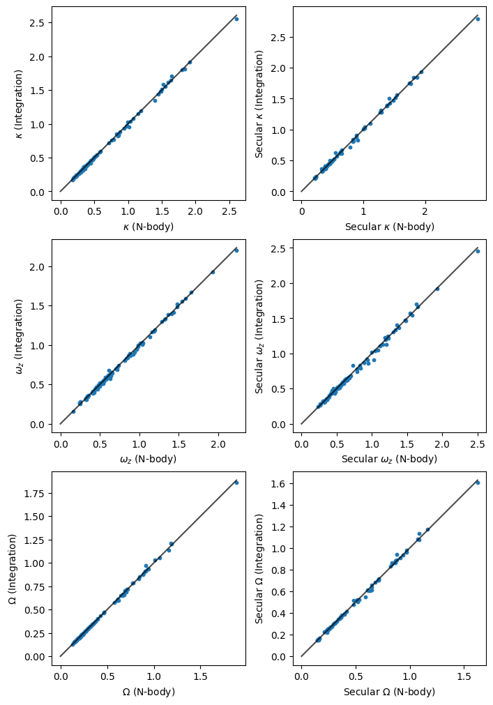
Comparison of frequencies for the set of orbits obtained from N-body simulations and integration in a fixed potential.
[11]:
fig, axes = plt.subplots(3, 2, figsize=(7,10), constrained_layout=True)

plot_comparison(axes[0,0], kappa, kappa_int, '$\\kappa$ (N-body)', '$\\kappa$ (Integration)')
plot_comparison(axes[0,1], kappa_sec, kappa_sec_int, 'Secular $\\kappa$ (N-body)', 'Secular $\\kappa$ (Integration)')
plot_comparison(axes[1,0], omegaz, omegaz_int, '$\\omega_z$ (N-body)', '$\\omega_z$ (Integration)')
plot_comparison(axes[1,1], omegaz_sec, omegaz_sec_int, 'Secular $\\omega_z$ (N-body)', 'Secular $\\omega_z$ (Integration)')
plot_comparison(axes[2,0], Omega, Omega_int, '$\\Omega$ (N-body)', '$\\Omega$ (Integration)')
plot_comparison(axes[2,1], Omega_sec, Omega_sec_int, 'Secular $\\Omega$ (N-body)', 'Secular $\\Omega$ (Integration)')
plt.show()

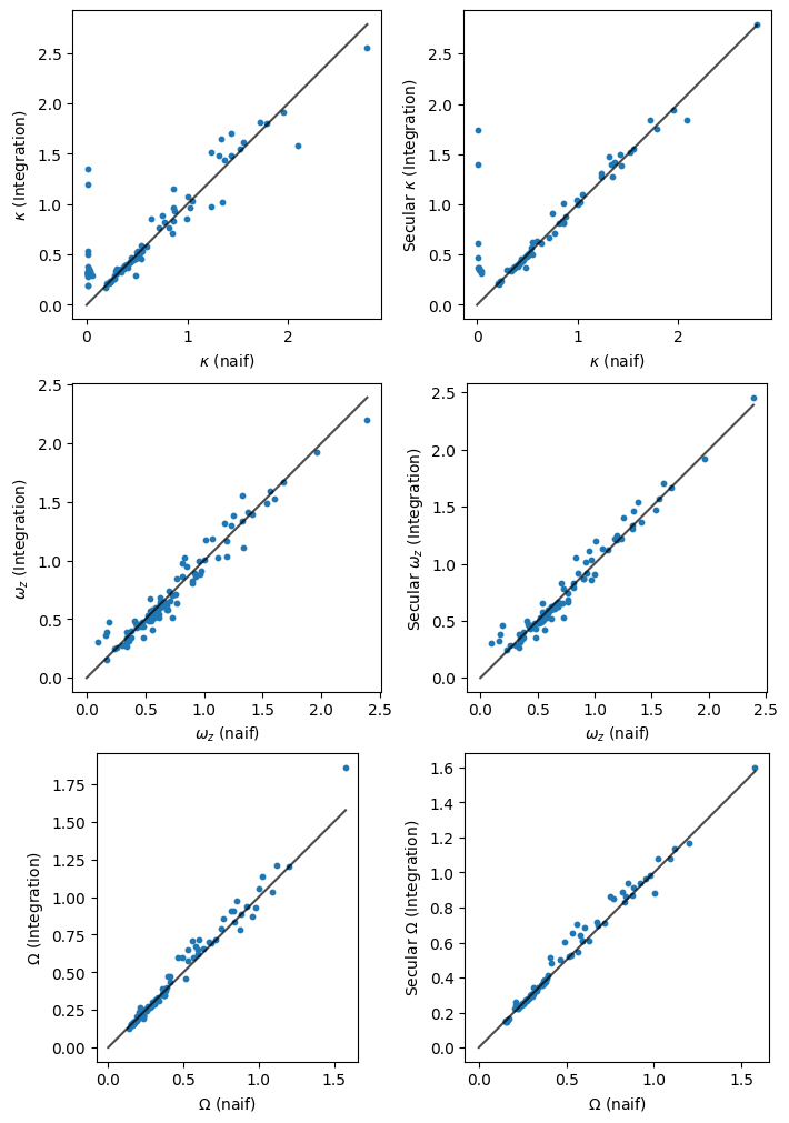
Comparison with frequency analysis naif
[12]:
%%time
freq_naif = OT.naif_frequency(parallel=True)

kappa_naif = np.abs(freq_naif[:,0])
omegaz_naif = np.abs(freq_naif[:,1])
Omega_naif = freq_naif[:,2]
CPU times: user 56.7 ms, sys: 81.8 ms, total: 138 ms
Wall time: 330 ms
[130]:
fig, axes = plt.subplots(3, 2, figsize=(7,10), constrained_layout=True)

plot_comparison(axes[0,0], kappa_naif, kappa_int, '$\\kappa$ (naif)', '$\\kappa$ (Integration)')
plot_comparison(axes[0,1], kappa_naif, kappa_sec_int, '$\\kappa$ (naif)', 'Secular $\\kappa$ (Integration)')
plot_comparison(axes[1,0], omegaz_naif, omegaz_int, '$\\omega_z$ (naif)', '$\\omega_z$ (Integration)')
plot_comparison(axes[1,1], omegaz_naif, omegaz_sec_int, '$\\omega_z$ (naif)', 'Secular $\\omega_z$ (Integration)')
plot_comparison(axes[2,0], Omega_naif, Omega_int, '$\\Omega$ (naif)', '$\\Omega$ (Integration)')
plot_comparison(axes[2,1], Omega_naif, Omega_sec_int, '$\\Omega$ (naif)', 'Secular $\\Omega$ (Integration)')
plt.show()